AP 186 Act14 - Image Compression

Nowadays storage capacities get bigger and grow faster so there's not much problem comparing it in the past where storage was an issue. Images were compressed to save storage space. In this activity, we'll explore about image compression using PCA or Principal Components Analysis.

In Fourier Transform, any signal can be represented by a sum of sinusoids (your basis functions) multiplied by coefficients. This concept of representing a signal with basis functions and proper coefficients is similar to PCA. In this case we will be doing it for images.

First I choose an image:

chosen image for this activity

and convert it to grayscale:

grayscale of the image

Then we cut up the image into 10 x 10 blocks and reshape this block into a 1-D array. We do this for the rest of the image and we'll have an n x p matrix where n is the number of 10 x 10 blocks and p is the number of elements per block (100 in this case). Next we apply PCA using the "pca" function in scilab.

correlation circle

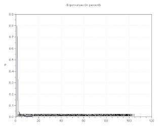
Eigenvalues

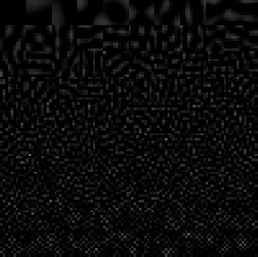
Eigenvectors

The "pca" function gives 3 output - the eigenvalues, the eigenvectors, and the coefficients. The image can be reconstructed from these and its quality depends on the number of eigenvectors used (i.e. the amount of compression).

And the reconstructions are:

using 1 out of 100 eigenvectors (cumsum of 80.5% for eigenvalues) (1.23 MB)

using 2 out of 100 eigenvectors. (cumsum of 85.5% for eigenvalues)Here the faces of the people are unrecognizable. (1.36 MB)

using 4 out of 100 eigenvectors. (cumsum of 91% for eigenvalues)Some faces begin to be a little recognizable (1.44 MB)

using 10 out of 100 eigenvectors (cumsum of 95.2% for eigenvalues) (1.46 MB)

using 48 out of 100 eigenvectors (cumsum of 99% for eigenvalues) (1.63 MB)

using all 100 eigenvectors (100%) (1.10 MB)

We can see that using only a few basis to reconstruct will result in a very poor and lossy quality of the image. The images using only 1, 2 and 4 eigenvectors look blocky and the high frequency features such as the faces are missing or blurred. As we increase the number of eigenvectors used, the quality becomes better and better and the minute features are showing up. At 10 eigenvectors the faces are quite recognizable and the image begins to look "ok". At 48 out of 100 eigenvectors the reconstructed image is decent and losses are not noticeable. Using all the eigenvectors, we get the same as the grayscale image. Also I should mention that when I used imwrite to save the images, the file size increases as i use more eigenvectors which is intuitive, however the file sizes are even bigger than the original image. And when all the the eigenvectors are used, the file size is the same as that of the original image.

What we did here was to use PCA on a grayscale image. True color images consists of 3 planes (RGB) and we tried applying PCA on each of the individual planes, and then adding them up in the end:

(cumsum of 95% for eigenvalues)

(cumsum of 99% for eigenvalues)

using all the eigenvectors for each plane (RGB)

As fewer eigenvectors are used, the image blurs and the colors also fade. However, there's a slight difference between the blue colors of the jacket in the reconstruction using all eigenvectors and the original image...maybe because of the scaling when using imwrite?

To grade myself I give a 10/10 for producing the required outputs as well as understanding the lesson about PCA and image compression.

Score: 10/10

Lastly I would like to acknowledge Dr Soriano, Arvin Mabilangan, Joseph Bunao, Andy Polinar, Brian Aganggan and BA Racoma for the helpful and insightful discussions. :D


- Dennis

References:
1. M. Soriano, "Image Compression"

AP 186 Act12 - Color Camera Processing

In this activity we will be playing around with the “white balance” setting of cameras and learn the concept behind it

Sometimes when we take pictures of colored objects, the color we see in the picture is different from the actual color of the object as we perceive it. The RGB values of an image is determined from the integral of the product of surface reflectance of the object, the spectral power distribution of the light source and the camera sensitivities and this is divided by the white balancing constant. It is due to this constant that white objects should appear white in the image.

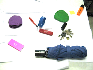
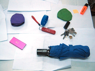
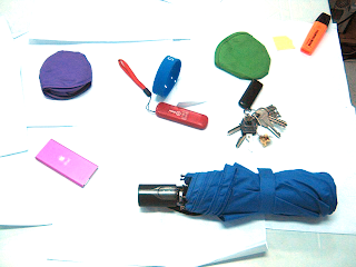
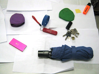
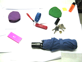
Most cameras have white balancing options such as: daylight, cloudy, tungsten, fluorescent and incandescent and the names pertain to the type of light source illuminating the object. We are first asked to take images of an ensemble of objects with colors representing major hues under a fixed light source and using different white balancing settings. I used BA Racoma’s Canon Powershot A480 camera with white balancing settings: daylight, cloudy, tungsten, fluorescent, and fluorescent_H. The objects used include: red USB, orange highlighter, yellow piece of paper, green fan sleeve, blue baller, indigo ipod, violet fan sleeve, purplish blue umbrella and a black USB. They were taken with a white background and under a fluorescent lamp.

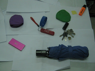
Image taken under "daylight" white-balancing setting

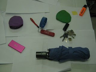
Image taken under "cloudy" white-balancing setting

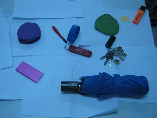
Image taken under "tungsten" white-balancing setting

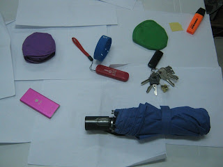
Image taken under "fluorescent" white-balancing setting

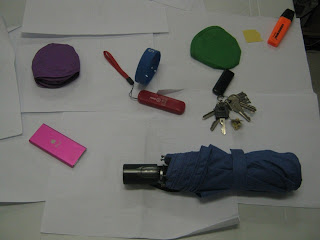
Image taken under "fluorescent_H" white-balancing setting

Shown above are the images taken with daylight, cloudy, tungsten, fluorescent and fluorescent_H white balancing setting. Under daylight, the image looks a bit more bluish while under cloudy, the image looks a bit… brownish. Fluorescent_H is almost like cloudy except that it looks more brownish or reddish. The image under the tungsten setting looks bluish since light from tungsten is very orange compared to daylight; the bluish white-balancing balances the orange tinge due to the tungsten bulb. The image looks best in fluorescent setting since the white background looks the whitest there.

We’ll try to white balance the wrongly balanced images. There are two methods of doing this: White Patch algorithm and Gray World algorithm. In White Patch algorithm we divide the RGB values of the image by the RGB values of a pixel from the image that we know is white respectively. Pixel values greater than 1 are clipped to 1. In Gray World algorithm, we take the averages of the R, G and B of the image and then use it as the divisor for RGB respectively. The white-balanced images are now:

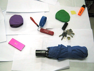
white-balanced (daylight) using White Patch algorithm

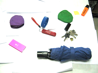
white-balanced (daylight) using Gray World algorithm

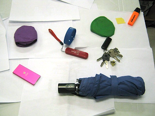
white-balanced (cloudy) using White Patch algorithm

white-balanced (cloudy) using Gray World algorithm

white-balanced (tungsten) using White Patch algorithm

white-balanced (tungsten) using Gray World algorithm

white-balanced (fluorescent_H) using White Patch algorithm

white-balanced (fluorescent_H) using Gray World algorithm

Wow!! White does really appear white here! It seems that as if a color overlay has been removed from the images and they now look brighter. The colors of the image became brighter and more vivid. Also, in the white-balanced images using the White Patch algorithm, I noticed that the area near the chosen pixel of a white object seems to be whiter or more saturated than the rest of the white background. Images that used the Gray World algorithm, meanwhile, appear more saturated. Perhaps this is because the majority of the pixels are white and thus when the average of the RGB values is taken and divided in their planes respectively, the image looks saturated.

Next we took another picture of an ensemble of objects having the hue along with a white object under a white-balancing setting that is not appropriate for the light source. In this case I used the tungsten setting and took the picture under the illumination of a fluorescent lamp. We then apply the White Patch algorithm and the Gray World algorithm independently and the results are:

Image taken under "tungsten" white-balancing setting

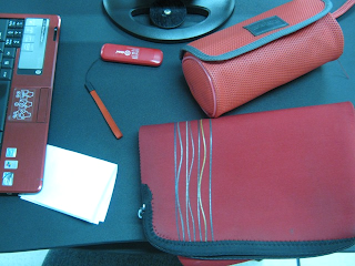
white-balanced using white patch algorithm

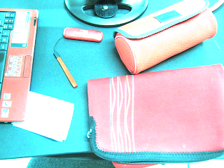
white-balanced using gray world algorithm

The balanced image using white patch algorithm looks almost the same as the original image, maybe because the white piece of paper may already look white. In the balanced image using gray world algorithm, the image once again looks saturated and moreover, it looks kind of bluish. But the white piece of paper does appear white though...

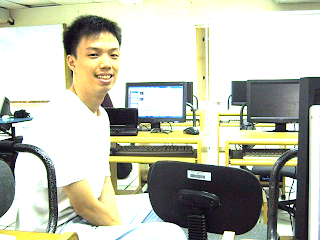
Aside from this BA Racoma played around with the custom white-balancing setting and took a picture of me with a deliberately wrong setting. So I applied the two algorithms once again and…

wrongly balanced image


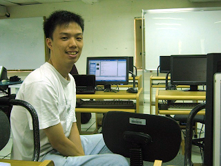
balanced using white patch algorithm


balanced using gray world algorithm

The original image looks greenish. After balancing with the white patch algorithm, the image looks a lot better with white being white. On the other hand, the balanced image using gray world algorithm looks saturated again, but white also appears white in the image. In my opinion the balanced image using white patch algorithm looks better although it's a bit dark. Balanced images using gray world algorithm also looks good except that it is too saturated. So if I were to pick one, I'd still pick the balanced image using white patch algorithm.

To grade myself, I give a 10/10 for understanding the lesson and producing the outputs required in this activity.

Score: 10/10

Lastly I would like to acknowledge Dr. Soriano and BA Racoma for the helpful discussions. Also, thanks to Mayanne Tenorio, Tisza Trono and BA Racoma for the materials used inthis activity.

References:

1. M. Soriano, "A12 - Color Camera Processing"

Appendix: (code)

// AP186 Color camera processing

// White patch algorithm
A = imread("C:\fluorescent_H.JPG");

R = A(:, :, 1);
G = A(:, :, 2);
B = A(:, :, 3);

// RGB values of pixel belonging to white
Rw = R(270, 160);
Gw = G(270, 160);
Bw = B(270, 160);

Rbal = R / Rw;
Gbal = G / Gw;
Bbal = B / Bw;

Rbal(find(Rbal > 1)) = 1;
Gbal(find(Gbal > 1)) = 1;
Bbal(find(Bbal > 1)) = 1;

A(:, :, 1) = Rbal;
A(:, :, 2) = Gbal;
A(:, :, 3) = Bbal;

imwrite(A, "C:\fluorescent_H_white_patch.PNG");

//imshow(A);

//Gray world algorithm
A = imread("C:\fluorescent_H.JPG");

R = A(:, :, 1);
G = A(:, :, 2);
B = A(:, :, 3);

// Get average value for R, G and B planes
Rw = mean(R);
Gw = mean(G);
Bw = mean(B);

Rbal = R / Rw;
Gbal = G / Gw;
Bbal = B / Bw;

Rbal(find(Rbal > 1)) = 1;
Gbal(find(Gbal > 1)) = 1;
Bbal(find(Bbal > 1)) = 1;

A(:, :, 1) = Rbal;
A(:, :, 2) = Gbal;
A(:, :, 3) = Bbal;

//imshow(A);
imwrite(A, "C:\fluorescent_H_gray_world.PNG");

---------------- end ----------------------

AP 186 Act13 - Color Image Segmentation

Sometimes in image processing, a Region Of Interest (ROI) needs to be isolated from the rest of the image. Thresholding is one way of doing it but when the color of the object or ROI is almost the same with the background, problems arise. Another way of doing it is through color image segmentation, which we will demonstrate in this activity.

First I pick an image with a single color and I chose this picture which i took:

picture of a Ferrari to be used for this activity

next we crop a region of interest that is monochromatic...

region of interest cropped from the front hood of the car

We first perform the parametric segmentation:
The ROI was loaded into scilab and the RGB colors were transformed into Normalized Chromaticity Coordinates (NCC) then from there the r and g values can be computed. After which we assumed independent Gaussian distributions in r and g and computed for their mean and standard deviation. From here the joint probability function is obtained and this criteria is used to segment the whole image. The result is a grayscale image:

parametric segmentation of the region of interest (the car)

and one can see that the red body of the car is isolated from the surroundings. The black spots near the front of the car are due to specular reflections in the image so they appear white and were not included. Even the reflection of the car from the glass window is included.

Next we perform another method which is the non-parametric segmentation. This method utilizes the 2D histogram of the r and g values in the ROI. So instead of computing the joint probability per pixel, the method looks up the it's value in the 2D histogram using the pixel's r and g values - backprojection in short. So from the r and g values of the ROI we made the 2D histogram:

2D histogram of r and g values of ROI

but since its origin is on the top left corner, we rotate this by 90 degrees by using mogrify function:

rotated 2D histogram of the ROI

normalized chromaticity space

and comparing this to the rg chromaticity diagram, the peak in the histogram coincide with the reddish part of the normalized chromaticity space which is correct since the ROI is reddish in color. Using this histogram, we performed histogram backprojection which is similar to activity 5 (Enhancement by histogram manipulation) and the result is:

non-parametric segmentation of the ROI (the car)

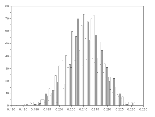
Comparing the results of the two methods, I would really have to say that the parametric method worked better at first glance. Nearly the entire body of the car is separated from the background while in non-parametric segmentation, the bumper as well as some other parts of the car are very faint. Although both methods were able to get the reflection of the car from the windows, the result from the parametric method seems to be better and more detailed. Looking at the 1D histograms of r and g value of the ROI...

histogram of r values of ROI

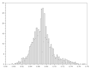
histogram of g values of ROI

no wonder the results of the parametric method were so good... we assumed r and g to have a gaussian distribution and looking at the histograms above, a gaussian distribution would be a good enough fit.

To grade myself, I give a 10/10 for comprehending the lesson and producing the required results.
Score: 10/10

Lastly I would like to acknowledge Dr. Soriano for helping me understand more about this activity.

References:
1. M. Soriano, "Color Image Segmentation"


Appendix: (code)

// AP186 Act 12 Color Image Segmentation

ROI = imread("C:\ROI.PNG");

// PARAMETRIC METHOD
// Compute per pixel the r and g values
R = ROI(:,:,1);
G = ROI(:,:,2);
B = ROI(:,:,3);

clear ROI;

divisor = R + G + B;

divisor(find(divisor==0)) = 1000000;

r = R ./ divisor;
g = G ./divisor;

clear R;
clear G;
clear B;

// Get mean and stdev of r ang g:
rmean = mean(r);
gmean = mean(g);
rstdev = stdev(r);
gstdev = stdev(g);


// For the whole image...
A = imread("C:\Ferrari_side_view.JPG");

// Compute per pixel the r and g values
R = A(:,:,1);
G = A(:,:,2);
B = A(:,:,3);

clear A;

divisor = R + G + B;

divisor(find(divisor==0)) = 1000000;

r = R ./ divisor;
g = G ./divisor;

clear R;
clear G;
clear B;

// Get their probabilities...
pr = 1/(rstdev * sqrt(2 * %pi)) * exp(-((r - rmean).^2)/(2*(rstdev^2)));
pg = 1/(gstdev * sqrt(2 * %pi)) * exp(-((g - gmean).^2)/(2*(gstdev^2)));

JP = pr .* pg;

//scf();
//imshow(JP, []);



//NON-PARAMETRIC METHOD
// Compute per pixel the r and g values
ROI = imread("C:\ROI.PNG");
R = ROI(:,:,1);
G = ROI(:,:,2);
B = ROI(:,:,3);

clear ROI;

divisor = R + G + B;

divisor(find(divisor==0)) = 1000000;

r = R ./ divisor;
g = G ./divisor;

clear R;
clear G;
clear B;

BINS = 32;
rint = round(r*(BINS-1) + 1); //ranges from 1 to 32
gint = round(g*(BINS-1) + 1);

colors = gint(:) + (rint(:)-1)*BINS;
hist = zeros(BINS, BINS);
for row = 1:BINS
for col = 1:(BINS-row+1)
hist(row, col) = length(find(colors==( ((col + (row-1)*BINS)))));
end;
end;

//scf();
//histmax = max(hist);
//X = hist/histmax;
//Y = mogrify(X, ['-rotate', '-90']);
//imshow(Y, []);

// For the whole image...
A = imread("C:\Ferrari_side_view.JPG");

// Compute per pixel the r and g values
R = A(:,:,1);
G = A(:,:,2);
B = A(:,:,3);

clear A;

divisor = R + G + B;

divisor(find(divisor==0)) = 1000000;

r = R ./ divisor;
g = G ./divisor;

clear R;
clear G;
clear B;

//Backproject
s = size(r);
rows = s(1);
columns = s(2);

S = zeros(rows, columns);

for i=1:rows
for j=1:columns
rvalue = r(i, j);
gvalue = g(i, j);
// round off since hist has only 32 bins
rint = round(rvalue*(BINS-1) + 1);
gint = round(gvalue*(BINS-1) + 1);
value = hist(rint, gint);
// replace pixel with the value
S(i, j) = value;
end;
end;

imshow(S, []);



--------------------------end-----------------------

AP186 Act11 - Playing notes by image processing

Just as the title suggests, we will be playing some notes by using image processing. A simple musical piece was selected where only one note is present in every column. This is again another activity where we have to integrate the skills and lessons learned from past activities.

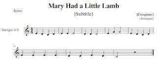
My selected piece was the nursery rhyme "Mary had a little lamb". (right hand only, no bass) Special thanks to Troy Gonzales for composing a copy for me. :)

music piece used for this activity

First I chopped up the image into two images, one for each line and they both have the same dimensions and as much as possible, the positions of the staves in the images are the same. Then their colors were inverted such that the notes are white and the background is black.

inverted and "chopped" version of the music sheet

My approach in detecting the notes is to correlate them with templates of different notes. Luckily, this piece has only two kinds of notes: quarter note and half note. So, templates of these notes where made with the note being white and the background being black.

quarter note and half note templates for matching

The 2 lines of the piece were loaded and binarized by determining the threshold from their grayscale histograms:

black and white version of the two lines of notes

Then their correlation with the quarter note and half note templates were taken. The result is a grayscale matrix and thresholding was once again done to reduce it into blobs. These blobs represent locations where there is a match. Afterwards these blobs were reduced into points or a single pixel for the next step - determining their relative locations from the staves.

line 1 correlated with the quarter note

line 1 correlated with the half note

black and white version of correlation of line 1 with quarter note

reduced to single pixels (line 1 corr w/ quarter note)

reduced to single pixels (line 1 corr w/ half note)

However, one problem encountered was that since the quarter and half notes differ by only just a little (shaded and not shaded), their correlation values with one another are high. Therefore when I used the quarter note template, all the quarter and half notes showed up. Adjusting the threshold didn't help as the true positives would disappear along with the false ones. Instead I remedied this by also taking the correlation with the half note and thresholding it such that only the quarter note showed up... and from these information, the type of note can be deduced.

The next task is to determine their relative vertical positions in order to determine their frequency. Due to the correlation, there is an offset between the position of the pixel from where the "body/blob" of the note should be. This is easily fixed by determining that offset. Also, the positions of the lines in the staves as well as the center of the spaces between them are taken. Then using an if-elseif-else statement, the relative positions of the notes can be determined. An error of +- 3 pixels is incorporated to compensate for the small fluctuations of the positions of the notes.

Finally, by combining the frequency of the note and it's timing (quarter or half), the piece can be played by the computer and the sound file is saved using wavwrite function. Here it is:

http://www.mediafire.com/?4wlr5qfjwba88at

Yay! :D

Lastly to grade myself, I give a 10/10 for being able to produce the required output and understand and integrate past lessons.

Score: 10/10

I would also like to thank Dr. Soriano, Arvin Mabilangan, Gino Leynes, Troy Gonzales, BA Racoma, Tisza Trono, Joseph Bunao for the very helpful discussions. :)


References:
1. M. Soriano, "A11 - Playing Notes by Image Processing
2. Physics of Music - Notes, (http://www.phy.mtu.edu/~suits/notefreqs.html) for the frequencies of the notes.


Appendix: (Code)
// AP186 Act11 Playing note by image processing

function n = note(f,t)
n = sin(2*%pi*f*t)
endfunction;


A1 = gray_imread("C:\maryline1.png");
T = gray_imread("C:\quarternote.png");

// threshold for A1 is determined to be 0.3
A1bw = im2bw(A1, 0.3);
Tbw = im2bw(T, 0.5);

// correlate with quarternote
FTA = fft2(A1bw);
FTT = fft2(Tbw);
FTAconj = conj(FTA);
B = fftshift(abs(fft2(FTAconj.*FTT)));

//threshold chosen to be 0.88
Bbw = im2bw(B, 0.88);

[L, n] = bwlabel(Bbw);

// To reduce blobs to dots
Bbwsize = size(Bbw);
quarternotecorr = zeros(Bbwsize(1), Bbwsize(2));
for i=1:n
[r, c] = find(L==i);
rc = [r' c'];
r = rc(:,1);
c = rc(:,2);
chalfvalue = c(int((length(c)+1)/2));
rhalfvalue = r(int((length(find(c==chalfvalue))+1)/2));
quarternotecorr(rhalfvalue, chalfvalue) = 1;
end

// correlate with halfnote
T = gray_imread("C:\halfnote.png");
Tbw = im2bw(T, 0.5);

FTT = fft2(Tbw);
B = fftshift(abs(fft2(FTAconj.*FTT)));

//threshold chosen to be 0.96
Bbw = im2bw(B, 0.96);

[L, n] = bwlabel(Bbw);

// To reduce blobs to dots
Bbwsize = size(Bbw);
halfnotecorr = zeros(Bbwsize(1), Bbwsize(2));
for i=1:n
[r, c] = find(L==i);
rc = [r' c'];
r = rc(:,1);
c = rc(:,2);
chalfvalue = c(int((length(c)+1)/2));
rhalfvalue = r(int((length(find(c==chalfvalue))+1)/2));
halfnotecorr(rhalfvalue, chalfvalue) = 1;
end

allnotes = halfnotecorr;

// To determine which ones are halfnotes
strel = ones(25,25);
quarternotecorr_dilated = dilate(quarternotecorr, strel, [13,13]);

[r c] = find(halfnotecorr==1);
rc=[r' c'];
len = length(rc(:,1));

halfnotecorr = zeros(Bbwsize(1), Bbwsize(2)); // reuse variables
for i=1:len
halfr = rc(i,1);
halfc = rc(i,2);
value = quarternotecorr_dilated(halfr, halfc);
if value == 0
halfnotecorr(halfr, halfc) = 1;
end
end

// Determine the positions of the blobs and timing
[L, Nnotes] = bwlabel(allnotes);
t_quarter = soundsec(0.25);
t_half = soundsec(0.5);
t_error = soundsec(3);

Cnote = 2*261.63;
Dnote = 2*293.66;
Enote = 2*329.63;
Fnote = 2*349.23;
Gnote = 2*392.00;

err = 3;
offset = 17; // determined from pics
Clvl = 86;
Dlvl = 80;
Elvl = 73;
Flvl = 66;
Glvl = 60;

s=[];

halfnotecorr_dilated = dilate(halfnotecorr, strel, [13,13]);

// BWLABEL IS NOT RELIABLE!!
[row, col] = find(allnotes==1);
n = length(row);

for i=1:n
r = row(i);
c = col(i);
valueQTR = quarternotecorr_dilated(r, c);
valueHLF = halfnotecorr_dilated(r, c);
r = r + offset;
if r >= (Dlvl + 3)
f = Cnote;
elseif r > (Elvl+3)
f = Dnote;
elseif r > (Flvl +3)
f = Enote;
elseif r >= (Glvl + 3)
f = Fnote;
else
f = Gnote;
end
if valueQTR == 1
t = t_quarter;
elseif valueHLF == 1
t = t_half;
else
t = t_error;
end
s = [s note(f, t)];
clear r;
clear c;
end




///////////////////////////////////////////////////////



// FOR THE 2ND LINE OF MARY HAD A LITTLE LAMB
A1 = gray_imread("C:\maryline2.png");
T = gray_imread("C:\quarternote.png");

// threshold for A1 is determined to be 0.3
A1bw = im2bw(A1, 0.3);
Tbw = im2bw(T, 0.5);

// correlate with quarternote
FTA = fft2(A1bw);
FTT = fft2(Tbw);
FTAconj = conj(FTA);
B = fftshift(abs(fft2(FTAconj.*FTT)));

//threshold chosen to be 0.88
Bbw = im2bw(B, 0.88);

[L, n] = bwlabel(Bbw);

// To reduce blobs to dots
Bbwsize = size(Bbw);
quarternotecorr = zeros(Bbwsize(1), Bbwsize(2));
for i=1:n
[r, c] = find(L==i);
rc = [r' c'];
r = rc(:,1);
c = rc(:,2);
chalfvalue = c(int((length(c)+1)/2));
rhalfvalue = r(int((length(find(c==chalfvalue))+1)/2));
quarternotecorr(rhalfvalue, chalfvalue) = 1;
end

// correlate with halfnote
T = gray_imread("C:\halfnote.png");
Tbw = im2bw(T, 0.5);

FTT = fft2(Tbw);
B = fftshift(abs(fft2(FTAconj.*FTT)));

//threshold chosen to be 0.995
Bbw = im2bw(B, 0.96);

[L, n] = bwlabel(Bbw);

// To reduce blobs to dots
Bbwsize = size(Bbw);
halfnotecorr = zeros(Bbwsize(1), Bbwsize(2));
for i=1:n
[r, c] = find(L==i);
rc = [r' c'];
r = rc(:,1);
c = rc(:,2);
chalfvalue = c(int((length(c)+1)/2));
rhalfvalue = r(int((length(find(c==chalfvalue))+1)/2));
halfnotecorr(rhalfvalue, chalfvalue) = 1;
end

allnotes = halfnotecorr;

// To determine which ones are halfnotes
strel = ones(25,25);
quarternotecorr_dilated = dilate(quarternotecorr, strel, [13,13]);

[r c] = find(halfnotecorr==1);
rc=[r' c'];
len = length(rc(:,1));

halfnotecorr = zeros(Bbwsize(1), Bbwsize(2)); // reuse variables
for i=1:len
halfr = rc(i,1);
halfc = rc(i,2);
value = quarternotecorr_dilated(halfr, halfc);
if value == 0
halfnotecorr(halfr, halfc) = 1;
end
end

// Determine the positions of the blobs and timing
[L, Nnotes] = bwlabel(allnotes);

halfnotecorr_dilated = dilate(halfnotecorr, strel, [13,13]);

// BWLABEL IS NOT RELIABLE!!
[row, col] = find(allnotes==1);
n = length(row);

for i=1:n
r = row(i);
c = col(i);
valueQTR = quarternotecorr_dilated(r, c);
valueHLF = halfnotecorr_dilated(r, c);
r = r + offset;
if r >= (Dlvl + 3)
f = Cnote;
elseif r > (Elvl+3)
f = Dnote;
elseif r > (Flvl +3)
f = Enote;
elseif r >= (Glvl + 3)
f = Fnote;
else
f = Gnote;
end
if valueQTR == 1
t = t_quarter;
elseif valueHLF == 1
t = t_half;
else
t = t_error;
end
s = [s note(f, t)];
clear r;
clear c;
end


sound(s);

--------------------------end----------------------------