AP 186 Act7 - Properties of the 2D Fourier Transform

For this activity, we'll explore some properties of the 2D Fourier Transform (FT):

Part A: Familiarization with FT of different 2D patterns
In this part, we created 2D patterns and then took their FT's and see what it looks like.

Square:

square pattern and its FT

Annulus (Donut):

Annulus pattern and its FT

Square annulus:

square annulus and its FT

Two slits along the x-axis symmetric about the center:

double slit pattern along x-axis and its FT

Two dots along x-axis symmetric about the center:

Two dots (1 pixel) along x-axis pattern and its FT

Note: If the dots are not of 1 pixel, a whole different FT pattern will appear:

different FT pattern if dots are not of 1 pixel

Part B: Anamorphic property of the Fourier Transform

First, we're asked to make a 2D sinusoid in the x direction (like a corrugated roof) and take it's FT:

sine wave (f=2Hz) and its FT

Next we change the frequency of the sinusoid:

f = 4 Hz

f = 8 Hz

f = 16 Hz

As the frequency of the sine wave is increased or decreased, the two peaks in the frequency space moves farther apart or closer together, respectively. This is because low frequencies are close to the center (zero) in frequency space and as you move away from the center, the frequency increases.

Adding a bias to the sinusoid and taking the FT:

sinusoid with bias and its FT

By adding the bias, the sinusoid now oscillates with non-negative values. However, we can see that there's an additional peak right in the middle of its FT. Digital images have no negative values so for example, what I can do to find the actual frequencies of the interferogram from Young's double slit experiment is to DC-filter it first. DC filtering will remove the bias and hence the middle peak in the FT. If the bias is non-constant, e.g. low frequency sinusoids, I can still get the frequencies of the interferogram by applying a high pass filter. This way, the low frequencies (the noise in this case), will be removed.

Next, we rotate the sinusoid and take its FT:

rotated 30 degrees

rotated 45 degrees

Rotating the sinusoid also amounts to rotating their FT by the same amount. This is a unique property of the 2D FT compared to the 1D FT.

Next, we created a pattern which is a combination of sinusoids in the X and Y direction, take its FT and see what it looks like:

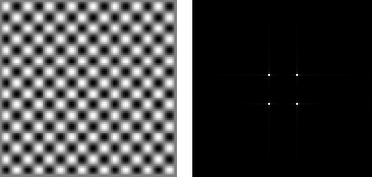
combination of sinusoids in the X and Y and its FT

Then we add several rotated sinusoids in the pattern. I added two sinusoids: 1 rotated by 30 degrees and another one rotated by 45 degrees. Since I know that rotating the sinusoids will also rotate their FT, the FT's of the added sinusoids individually are shown in the last part. At first I predict that adding the sinusoids would result in a rotation of the FT of the "eggcart". But remembering that the FT is a linear transformation, the FT of the result should be the addition of the FT's of the components. Therefore, the resulting FT should be something like 4 peaks on the corners of a square, then two peaks tilted at 30 degrees and another 2 peaks tilted 45 degrees. Checking this prediction:


Indeed, the resulting FT is the same as the prediction! :D


Rating myself, I would give myself a 10/10 for understanding the lesson and producing the required outputs.

Score: 10/10

Lastly, I would like to acknowledge Dr. Soriano, BA Racoma and Androphil Polinar
for the helpful discussions.

- Dennis

References:
1. M. Soriano, "A7 - Properties of the 2D Fourier Transform"

AP 186 Act6 – Fourier Transform Model of Image Formation

In this activity we will be dealing with Fourier Transforms (Fast Fourier Transforms) and their applications in image processing. Cooley and Tukey made the FFT algorithm and it’s widely used in image as well as signal processing.

Part A. Familiarization with FFT

First we’re asked to make a white circle centered on a black background:

(Note that this circle can also represent a circular aperture. I’ve made my circle smaller since this will result in a bigger Airy disk as will be seen later.)

Then we converted this to grayscale and performed the Fast Fourier Transform (FFT). Abs() was used to get the intensity values since the FFT will return an array of complex numbers.

I = imread('C:\circle.PNG');
Igray = im2gray(I);
FIgray = fft2(Igray);
imshow(abs(FIgray), []);

And this is the result:

FFT of the white circle

It looks like a pure black picture but take a look at the four corners. :p

This is a result of the FFT. It’s fast, but it also results in the reversal of the quadrants diagonally. Therefore, applying the fftshift will give:

imshow(fftshift(abs(FIgray)), []);

shifted FFT of the circle

Now that’s better. :) That’s the Fourier transform of the white circle.

Applying the FFT again on the transformed image (or consequently, applying the FFT twice on the original image) will theoretically result in an inverted original image:

imshow(abs(fft2(FIgray)));

circle FFT'ed twice

Well, we got the original image alright. But we can’t tell if this is inverted since an inverted circle is still a circle. So we try this on the letter “A”:

The (unshifted) FFT of A:

I = imread('A.bmp');
Igray = im2gray(I);
FIgray = fft2(Igray);
imshow(abs(FIgray), []);

unshifted FFT of "A"

And applying fftshift:

imshow(fftshift(abs(FIgray)), []);

shifted FFT of "A"

And that’s the Fourier transform of “A”.

Now applying the FFT twice… we get:

imshow(abs(fft2(FIgray)));

"A" FFT'ed twice

Which is indeed, the inverted image of the letter “A”. :D An inverted image results in the application of FFT twice because doing so will result in the introduction of a negative sign in the x’s and y’s. If you want to get your original image back from a Fourier transformed image, do the inverse Fourier transform. :)

Part B. Simulation of an imaging device

We’re asked to create an image of the letters “VIP” and this will be our object to be imaged. I used Arial font because according to the activity manual, sans serif fonts are sharp.

object

We also created a white circle on a black background and this represents the aperture of a lens.

aperture

The image of the “VIP” can be obtained by convolving the object with the transfer function of the imaging system. Convolution is done by taking the product of the FFT of the grayscaled object with the fftshifted aperture and then inverse fourier transforming. The aperture image doesn’t need to be FFT-ed because it is already in the Fourier Plane.

T = gray_imread('C:\VIP.bmp');
A = gray_imread('C:\circle.PNG');
Ar = fftshift(A);
Ta = fft2(T);
FRA = Ta.*Ar;
IRA = fft2(FRA);
imshow(abs(IRA), []);

The output is:

r = 0.7

Note that it is inverted and this is true for real images.

Making the size of the aperture smaller, we get…

r = 0.4

r = 0.25

r = 0.1

The image quality reduces when the lens aperture becomes smaller and smaller because less and less rays are able to pass through it. The more rays the lens can collect, the better the image quality.

Part C. Template Matching using correlation

Template matching is basically a type of pattern recognition in which it will determine matches between the test object and the template.

For this part, we created the white texts in black background of: “THE RAIN IN SPAIN STAYS MAINLY IN THE PLAIN.”

text

and our template will be the letter “A” with the same font style and size as in our text:

template

We get the correlation of these two by multiplying the FT of A and the conjugate of the FT of the text and then inverse Fourier transforming by using ifft().

T = gray_imread('C:\text.PNG');
A = gray_imread('C:\A.bmp');
FT = fft2(T);
FA = fft2(A);
FTconj = conj(FT);
FRA = FA.*FTconj;
IRA = ifft(FRA);
imshow(abs(IRA), []);

This is what I got:

correlation of text and template using ifft

It looked like the quadrants were reversed diagonally so I applied the fftshift after inverse FT-ing:

imshow(fftshift(abs(IRA)), []);

shifted correlation

Now it looks inverted… so I tried using the fft2 instead of ifft:

IRA = fft2(FRA);

imshow(abs(IRA), []);

correlation of text with template using ifft2

and fftshifting…

imshow(fftshift(abs(IRA)), []);

shifted correlation

Now this looks more correct. The original text could be made out from this image but there seems to be bright spots were the letter “A” is present. Therefore the bright spots represent a match since these are the positions were the correlation is highest.

I thought… what if the template is a “P” and there are “B”’s in the text… what would happen? So I made my own text:

text 2

And my own template:

template 2

And the correlation is…

limitation of method

It can be seen that despite there is only one capital “P”, there are multiple bright spots. This is because the other letters like “B” looks very similar to P except that it has an extra part at the bottom. The other letters also have parts that are similar to “P” so they have a high correlation. Therefore this shows the limitation of the technique.

Part D. Edge detection using the convolution integral

We were asked to make a 3x3 matrix pattern of edges such that the sum of all the elements is zero. Then we convolved this with the "VIP" image using imcorrcoef():

For the matrix:

[-1 -1 -1

2 2 2

-1 -1 -1]

We get:

convolved image

We can see that the horizontal edges of the image are brighter. Also note that the matrix has the same values horizontally. What this does it that it scans the image and tries to match its edges with the matrix.

For the vertical matrix:
[-1 2 -1
-1 2 -1
-1 2 -1]

We get:

convolved image

This time, the vertical edges of the image are brighter :D

For the spot pattern:
[-1 -1 -1
-1 8 -1
-1 -1 -1] :

convolved image

This time, all of the edges of the image are bright. This is because in the pattern, all of the edges have the same value.

The code for this is:

T = gray_imread("C:\VIP.bmp");

pattern = [-1 -1 -1; 2 2 2; -1 -1 -1];

F = imcorrcoef(T, pattern);

imshow(F, []);

And that wraps up the activity. :)

For the score, I give myself a 10/10 for producing the required output and understanding the lesson. Plus 2 points for testing the limitations of the technique of correlation, which gives a total of...

Score: 12/10

Lastly, I would like to acknowledge Dr. Soriano for the helpful discussions. :D


- Dennis

References:
1. M. Soriano, "A6 - Fourier Transform Model of Image Formation"

AP 186 Activity 5: Enhancement by Histogram Manipulation

In this activity we will be modifying the histogram of the image in order to enhance its quality and improve certain image features. This can be done by mapping the graylevel values of the image such that the new image will have the desired cumulative distribution function (CDF).

I've chosen this picture:


and I ran the following code in Scilab:

stacksize(10000000);
A = gray_imread("C:\test1.jpg");
B = tabul(A, "i");
B1 = B(:,1);
B2 = B(:,2);
size(A);
s = 540*720;
B2norm = B2/s;
B2cumsum = cumsum(B2norm);
A1d = A(:);
yCDF = interp1(B1, B2cumsum, A1d);
xdesired = interp1(B1, B1, yCDF);
Aedited = matrix(xdesired, [540, 720]);
imwrite(Aedited, "C:\test1modified.png");

Basically what this code does is it loads the image into scilab, then it gets the image's normalized histogram and CDF. Then, it interpolates in order to get the y values in the image's CDF. After that it interpolates once again in order to get the grayscale value having this CDF value in the desired CDF. All the pixels in the image are backprojected and replaced by the x-values of the desired CDF.

In this case, the desired CDF is a line with slope = 1, that is, its PDF is just a uniform distribution. Executing the code above, I get:

histogram of the image (not normalized)

normalized histogram of the image

Histogram equalized image


Original grayscaled image

and comparing the CDF's before and after:

CDF before enhancement

CDF after enhancement


PDF after enhancement

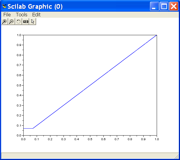
It is noticeable that the modified image has a higher contrast than the original. The light colored pixels seem to become lighter and the dark pixels seem to become darker. It also looks like that the "gray fog" over the original picture has been removed. The image is called histogram equalized image because we have modified its histogram such that every gray level the original image possess now have equal probability. Thanks to this, the picture is now brightened up a bit. :)

Also, the CDF of the enhanced image is a straight line and that was our desired CDF. Note that there's a small horizontal segment. This is because in the histogram of the original image, there's a range of grayscale values where no or very little pixels possess. This can also be seen in the modified PDF.

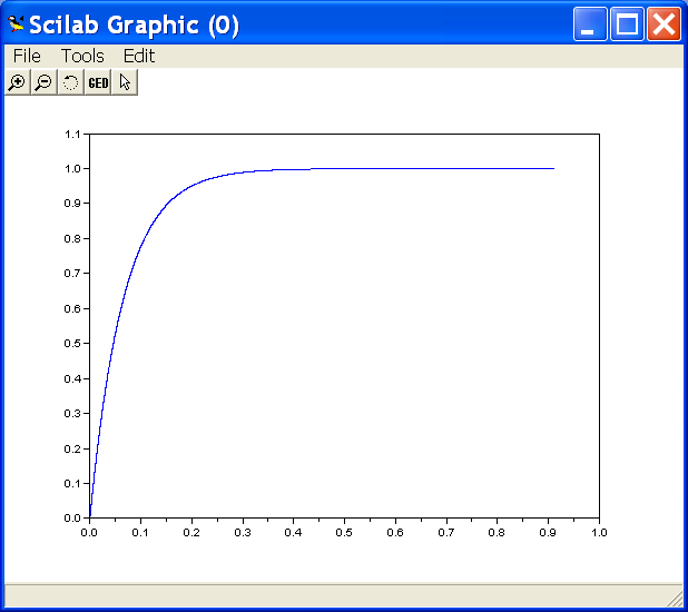
Next, I tried the technique on different CDF's. The first one is normal distribution: (mean = 0.5, std = 0.1)

histogram of normal distribution


CDF of normal distribution

The code was slightly changed:

A = gray_imread("C:\test1.jpg");
B = tabul(A, "i");
B1 = B(:,1);
B2 = B(:,2);
size(A);
s = 540*720;
B2norm = B2/s;
B2cumsum = cumsum(B2norm);
A1d = A(:);

y = grand(1, s, 'nor', 0.5, 0.1);
C = tabul(y, "i");
C1 = C(:,1);
C2 = C(:,2);
C2norm = C2/s;
C2cumsum = cumsum(C2norm);

yCDF = interp1(B1, B2cumsum, A1d);
xdesired = interp1(C2cumsum, C1, yCDF);
Aedited = matrix(xdesired, [540, 720]);
imwrite(Aedited, "C:\test1modified.png");

And the resulting image is:

Histogram manipulated image

Original image

Personally, I don't think using the histogram manipulated image is of better quality than the original image; it looks more hazy and less contrasted than the original. This is because for the normal distribution, most of its elements are concentrated near the mean and the standard deviation used here is quite small, meaning the pixels are concentrated around a range of graylevel values, which explains image's low contrast.

Like our first case, the histogram and CDF of the modified image resembles the desired one:

histogram of modified image


CDF of modified image

Next, I tried the exponential distribution:

Histogram of exponential distribution


CDF of exponential distribution

And the result is:

histogram manipulated image

original image

The manipulated image appears a lot darker than the original image because due to the exponential distribution, the pixels are concentrated at the left of the histogram, meaning there are now more pixels having darker values.

And the histogram and CDF of the modified image are:

histogram of manipulated image

CDF of manipulated image

Lastly, I used Photoshop to manipulate the histogram of the image:

Using Photoshop to manipulate the CDF

histogram manipulated image


original image

The image now is of higher contrast and it looks better! For me, its quality is better than the other histogram manipulated images. :D

For the score, I give myself 10/10 for understanding the lesson and being able to produce the requirements.

Score: 10/10

Finally, I would like to thank Dr. Soriano, Joseph Bunao, Arvin Mabilangan, BA Racoma, and Andy Polinar for the insightful and helpful discussions.

References:
1. M. Soriano, "A5 - Enhancement by Histogram Manipulation"