What we did is to try to predict the results of:
1. 5 x 5 square
2. A triangle, base = 4 boxes, height = 3 boxes
3. A hollow 10 x 10 square, 2 boxes thick
4. A plus sign, one box thick and 5 boxes along each line.
when dilated and eroded with:
a. 2 x 2 ones
b. 2 x 1 ones
c. 1 x 2 ones
d. cross, 3 pixels long, 1 pixel thick
e. A diagonal line, two boxes long: [0 1, 1 0].
and see if our results match when this is done via scilab.
The origin for the structuring element is (1, 1) if it can fit in a 2 x 2 array. If the (1, 1) element is not present, then the center will be (2, 1). For the cross, the center is located at its center.
Now, the following are the results:
Dilation:
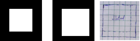
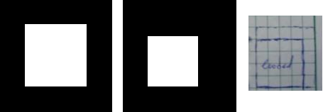
5 x 5 square dilated/eroded by a, b, c, d and e:
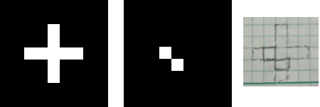
Left figure shows the original image, middle figure shows dilated/eroded image using scilab, right figure shows predicted image after dilation/erosion.
2 x 2 ones:
dilation:
dilation:
 erosion:
2 x 1 ones:
dilation:
 erosion:
1 x 2 ones:
dilation:
 erosion:
cross:
dilation:
 erosion:
diagonal line:
dilation:

erosion:
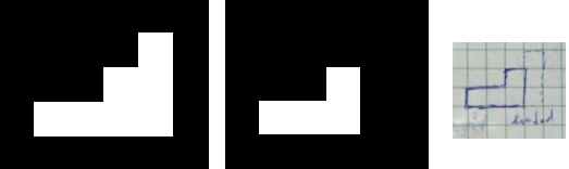
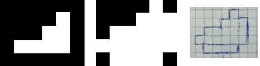
Triangle dilated/eroded by a, b, c, d and e:
2 x 2 ones:
dilation:

erosion:

2 x 1 ones:
dilation:

erosion:

1 x 2 ones:
dilation:

erosion:
cross:
dilation:
erosion:

diagonal line:
dilation:

erosion:

Hollow 10 x 10 square dilated/eroded by a, b, c, d and e:
2 x 2 ones:
dilation:

erosion:

2 x 1 ones:
dilation:

erosion:

1 x 2 ones:
dilation:

erosion:

cross:
dilation:

erosion:

diagonal line:
dilation:

erosion:

Plus sign dilated/eroded by a, b, c, d and e:
2 x 2 ones:
dilation:

erosion:

2 x 1 ones:
dilation:

erosion:

1 x 2 ones:
dilation:

erosion:

cross:
dilation:

erosion:

diagonal line:
dilation:

erosion:
As seen, the predictions match the outcomes from scilab. Yay! :D
Next, we explore other morphological operations available in scilab such as thin and skel:
The "thin" function utilizes the Zhang-Suen technique. Compared to the "skel" function, the output of the thin are not always connected. The Zhang Suen technique contains two sub-iterations, and it removes pixels if those pixels satisfy conditions such as connectivity, number of neighbors and the configuration of certain neighbors (on or off). The output of the "thin" function is an internal skeleton of the image which is capable of representing the shape and orientation of the original. It deletes the border of the image. As seen in the figure below, the sample image is "thinned" indeed.
 Sample image (left) and the result after "thinning" (right)
"skel" on the other hand, outputs three matrices (for scilab) - the grayscale skeleton image, the Euclidean distance transform of the image, and the discrete Voronoi Diagram of the boundary pixels. Thresholding can be applied to the grayscale skeleton system in order to get the binary skeleton of variable thickness depending on the threshold. The "skel" function is somewhat like a subset or a special case of "thinning" since getting the skeleton of an image involves thinning it down. And as mentioned earlier, the "skel" function will produce a connected skeleton.
 from left to right: sample image, its grayscale skeleton image, euclidean distance transform image, and its discrete Voronoi diagram.
Finally, I give myself a score of 10/10 for understanding the lesson and being able to (accurately) predict the dilation/erosion of the images as well as produce the required output.
Score: 10/10
Lastly, I would like to acknowledge Dr. Soriano, Cheryl Abundo, Arvin Mabilangan, and BA Racoma for the insightful discussions that made me understand more about the techniques. :D
- Dennis
References:
1. M. Soriano, "Morphological Operations"
2. http://www.rupj.net/portfolio/docs/skeletonization.pdf
3. http://www.mathworks.com/access/helpdesk/help/toolbox/images/bwmorph.html
Appendix: (Code, note, some semi colons are removed because it messes with the formatting)
// Square
nx = 9; ny = 9; //defines the number of elements along x and y
x = linspace(1,9,nx); //defines the range
y = linspace(1,9,ny);
[X,Y] = ndgrid(x,y); //creates two 2-D arrays of x and y coordinates
A = ones(nx,ny);
A(find(X<3))>7)) = 0;
A(find(Y<3))>7)) = 0;
// Triangle
nx = 5; ny = 6; //defines the number of elements along x and y
x = linspace(1,5,nx); //defines the range
y = linspace(1,6,ny);
[X,Y] = ndgrid(x,y); //creates two 2-D arrays of x and y coordinates
A = zeros(nx, ny);
A(find(X>3)) = 1;
A(2, 5) = 1;
A(3, 4) = 1;
A(3, 5) = 1;
A(find(X>4)) = 0;
A(find(Y<2))>5)) = 0;
// Hollow 10x10 square
nx = 14; ny = 14; //defines the number of elements along x and y
x = linspace(1,nx,nx); //defines the range
y = linspace(1,nx,ny);
[X,Y] = ndgrid(x,y); //creates two 2-D arrays of x and y coordinates
A = zeros(nx, ny);
A(find(X<5))>10)) = 1;
A(find(Y<5))>10)) = 1;
A(find(X>12)) = 0;
A(find(X<3))>12)) = 0;
A(find(Y<3)) nx =" 9;" ny =" 9;" x =" linspace(1,nx,nx);" y =" linspace(1,nx,ny);" a =" ones(nx,">5)) = 0;
A(find(X<5)) = 0;
A(3, 5) = 1;
A(4, 5) = 1;
A(6, 5) = 1;
A(7, 5) = 1;
A(5, 1) = 0;
A(5, 2) = 0;
A(5, 1) = 0;
A(5, 9) = 0;
A(5, 8) = 0;
scf();
imshow(A,[]);
2x2
SE = [1 1; 1 1];
2x1
SE = [1; 1];
1x2
SE = [1 1];
cross
SE = [0 1 0; 1 1 1; 0 1 0];
diagonal
SE = [0 1; 1 0];
R2 = erode(A, SE, [2, 1]);
R1 = dilate(A, SE, [2, 1]);
scf();
imshow(R1, []);
scf();
imshow(R2, []);
R3 = thin(A);
scf();
imshow(R3, []);
[R4, R5, R6] = skel(A);
scf();
imshow(R4, []);
scf();
imshow(R5, []);
scf();
imshow(R6, []);