Sunday, June 27, 2010

AP 186 Activity 4: Area Estimate of Images with Defined Edges

The objective of this activity is to be able to estimate the area of images that have defined edges using Green's theorem.

First, we're asked to make a black and white image of a regular object with the object being white and the background colored black. The area of the object must be known in order to compare it with the results. So I made this 150 by 80 pixel white rectangle with it's upper left corner starting at 100, 100 (origin at upper left corner) using Paint.

white rectangle (150 x 80 pixels)

And as told, I saved it in BMP format rather than JPG. So the white rectangle has an area of 150 x 80 = 12,000 pixels.

Next, let's load this into scilab and compute for the area:
I = imread("C:\shape.bmp");
[x, y] = follow(I);
xiplus1 = x;
d = xiplus1(1);
xiplus1(1) = [];
xiplus1(452) = d;
yiplus1 = y;
e = yiplus1(1);
yiplus1(1) = [];
yiplus1(452) = e;

A = 0.5 * sum((x .* yiplus1) - (y .* xiplus1))
The removal and addition of the 1st and last elements on xiplus1 and yiplus1 are just to shift it one place. x and y contains 452 elements. And fortunately, the follow function gives out the parametrized contour vectors x and y, so x and y are in coordinate system (not rows and columns).

I got the answer of 11,544 pixels which has a 3.8% error:It's a good estimate since the error's under 5%; it's a fairly accurate technique. Although personally, I was expecting it to perform better since the shape was a simple rectangle.


Now let's try the area estimation on a real location. Using Google maps, I picked the Quezon City Circle, which is bounded by the Elliptical road.

Image of Quezon City circle taken from Google Maps (click to zoom in)

Then using paint, I delineated the area of interest from the rest and the result was:

Area of interest with the edge delineated

Now using the same procedure as done above, I got the answer of 50, 549.5 pixels. In order to convert this into square meters, I use the technique in Activity 1 to determine the conversion factor from pixels to meters from the scale in Google maps.

scale bar on the bottom left corner (click to zoom in)

I have determined that 87 pixels = 200 meters (lengthwise). So that means 1 lengthwise pixel = 2.299 meters and 1 (square) pixel = 5.285 sq meters. Therefore 50, 549.5 pixels would be equivalent to:
267, 139.65 sq meters
Now's let's try to compute for the error. Since the scale bars take up two pixels:

scale bar

This means that the error would be plus/minus 1 pixel (lengthwise), which would translate to: (using error propagation)

(200/87) * (1/87) = 0.0264 meters.

Therefore the error in area per pixel would be:

(200/87)*(2)*(0.0264)*(87/200) = 0.121 sq meters

Multiplying this with our answer with 50, 469 pixels, we get the error of:
6106.75 sq meters
which is 2.29% of the result.

So the final answer is:
267, 139.65 +- 6106.75 sq meters
Finally I have to compare this with the actual value. Sadly, I can't find the area of the region inside the elliptical road on the internet so Joseph Bunao and I used Google Earth to determine the semi-major and semi-minor axis of the ellipse.

Finding the length of semi-major and of semi-minor axis

And we have determined 328.37 m and 259.65 m to be the lengths of the semi-major axis and semi-minor axis respectively. Using the formula for the area of an ellipse, we get the value:
267, 856.18 sq meters
Wow! The estimated area is very close to this value and has an error of 0.27%. This shows that the technique is accurate when dealing with images with defined edges since this will determine the contour that is used in Green's theorem.

And with that, I give myself a 10/10 for producing the requirements and understanding the lesson. The images are clear and of good quality.

Score: 10/10

Lastly I would like to thank Dr. Soriano for always entertaining my questions and Joseph Bunao for helping me find the lengths of the axes of the elliptical road.

- Dennis

References:
1. M. Soriano, "A4 - Area Estimation"
2. Google Maps

Thursday, June 24, 2010

AP 186 Activity 3: Image Types and Formats

This time, we'll be exploring different image types and formats such as jpg, png, gif and tiff.

This activity also requires us to show examples of basic image file types as well as advanced image file types:

Basic types:

1. Binary images taken from http://emis.math.ecnu.edu.cn/journals/EJC/Surveys/ds5/gifs/rot6.gif

2. Grayscale images
3. Indexed images taken from sample pictures of Adobe Photoshop CS3
this one is both a grayscale image and an indexed image
4. Truecolor images photo by Denille Teh of her dog


Advanced image file formats:

1. High dynamic range (HDR) imagestaken from http://studioshadowlight.com/images/uploads/HDR.jpg

2. Multi or hyperspectral imagetaken from http://gdsc.nlr.nl/gdsc/sites/default/files/images/multispectral/ik_beijing_c_big.jpg

3. 3D imagestaken from http://www.callipygian.com/3D/corpseplant.jpg

4. Temporal images or Videos

taken from R.T. Hanlon, A.C. Watson and A. Barbosa in "A 'Mimic' Octopus' in the Atlantic: Flatfish Mimicry and Camouflage by Macrotritopus defilippi" published in Biol. Bull. 218: 15–24.(February2010)

Now let's see what kind of image is the scanned figure from Activity 1:

But oops, I had to increase the stack size of scilab first with the command:

stacksize(10000000);
once that's done,based on the matrix size, the scanned figure is saved as a truecolor image.

Now let's convert a truecolor image into grayscale and black and white :)
We'll use this truecolor image.
540 x 720 x 3
Using the code:
I = imread("C:\image1.jpg");
J = im2gray(I);
imshow(J)
and
I = imread("C:\image1.jpg");
J = im2bw(I, 0.5);
imshow(J)
(0.5 is the threshold level; the fate of the pixel turning black or white depends if it exceeds this value)

we get:and their matrix sizes are both

540 rows by 720 columns
note that the third channel (for RGB) disappeared.

The next part of the activity is to use the histogram to set the threshold for the conversion of the scanned graph into black and white.

However, I keep getting the error:
!--error 17
stack size exceeded! (Use stacksize function to increase it)
even though I set the stacksize to a big value and resized my picture into a lower resolution. So I asked Cheryl Abundo to grayscale it for me. (Thank you!)Using the histplot function:

histplot(256, I)

I chose the threshold to be 220/256 = 0.859375 and converted it to black and white...The lines have been separated from the background but there's this huge black blob at the left side due to the quality of the scan. The dark part at the left side is as the lines so they also appear even though a threshold has been applied.

This activity also requires us to research about the different image file formats so here goes...

Let's start with...

JPEG - Joint Photographic Experts Group
This is one of the most famous and used image file formats because of it's ability to compress the file. However, it uses lossy compression most of the time meaning some information is lost due to compression. Most digital cameras also save in this format. JPEG or JPG is advantageous in applications where image size is more valued than quality. JPEG supports 8 bits per color (for R, G and B) for a total of 24 bits. It also supports grayscale of 8 bits.

GIF - Graphics Interchange Format
This format supports up to 8 bits of color for a total of 256 colors. This format is suitable for small images with only a few colors such as logos. Also, most animated pictures are saved in this format. GIF uses lossless LZW compression. This file format was introduced by CompuServe to display 8 bit color images online.

PNG - Portable Network Graphics
Basically, this format is developed to replace the GIF. It is free and open source and supports truecolor (16 million colors). PNG files are typically bigger than JPG files since it uses lossless ZIP compression. Also like GIF, PNG is more effective in images with big solid colors and slowly varying colors.

TIFF - Tagged Image File Format
This format can support 8 bits per color (24 bits) as well as 16 bits per color (48 bits). It's compression can by either lossy or lossless. This format is preferred in saving documents for archiving. It also uses LZW lossless compression. LZW is the acronym for Lempel-Ziv-Welch, named after Israeli researchers Abraham Lempel and Jacob Zif. Because of it's lossless compression and quality, it has a high file size. This is also used in medical images.

BMP - BMP file format
This format is also called bitmap and is developed for storing images and graphics in the Windows operating system hence they are easily recognizable in Windows.

References:
1. M. Soriano, "A3 - Image Types and Formats"
2. Wikipedia - Image file formats (http://en.wikipedia.org/wiki/Image_file_formats#JPEG.2FJFIF)

3. http://www.scantips.com/basics09.html


Lastly, I'll grade myself a score of 10/10 for being able to produce the requirements and understand the lesson. No bonus points for me this time :(

Score: 10/10

I would like to once again acknowledge Dr. Soriano for her guidance and Cheryl Abundo for converting the scanned graph into grayscale for me.

- Dennis

Tuesday, June 22, 2010

AP 186 Activity 1: Digital Scanning

*Transferred from Facebook notes to here*

This blog is for one of our major subjects: Applied Physics 186 which requires us to write blog reports about our activity. So if you're reading this to find out what my favorite food is or what crazy things I did today, you're not gonna find it. =p

So let's start:

Activity 1 - Digital Scanning


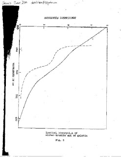
Basically the objective of this activity is to get any hand-drawn graph from any journal article (which means the journal has to be old, since they use computers to graph nowadays), scan it, then reproduce the graph in Microsoft Excel using ratio and proportion of the pixels and their corresponding physical value. We get bonus points if we are able to overlap the two graphs together for a better comparison.

I found this nice looking graph in the CS lib from the article:

The Photographic Processes in Spectrum Analysis by B. H. Carroll
Applied Spectroscopy, Vol. 1, Issue 4, pp. 1-15 (1946)

I chose the graph because:
  1. It's big.
  2. It's smooth.
  3. It's not in log scale and
  4. It has two curves in it. :)

I don't have a scanner so I asked my friend Millicent Singson to scan it for me. (Thank you!) The scanned picture has the dimensions 1700 x 2200 pixels.


The picture is a bit tilted so I used Adobe Photoshop to rotate it.

In order to reproduce the graph, I have to find an equation relating pixel location to physical values. So for the x and y axes, I got the pixel location of the start and end values of axes. Then the "multiplier" would be:

(End value - Start value)/(End Pixel - Start Pixel)

which we will denote as Mx and My for the x and y axis repectively.

Then you just have to multiply this to the pixel location and you would get the value. However, since i didn't crop the picture before i started counting the pixels, the pixel locations would not start at 0. Therefore I would have to subtract this "pixel offset" first before multiplying it with the above equation.

Another problem is that the origin (0, 0) doesn't start at the bottom left corner but rather at the top left corner. But this can be easily solved. :)

Another thing to keep in mind is to add the initial starting value of the axis after you convert from pixel to value. In this case, I added 200 to the values in the x axis.

So the equation is:

(x pixel location - x pixel offset) * Mx + x value offset

for the x axis and

(y pixel location - y pixel offset) * My + y value offset

for the y axis

I got plenty of sample points (17 for the blue curve and 20 for the red curve) and reconstructed it. After overlaying the image with the graph, there's a discrepancy between the tick marks of the two. Eventually I found out that the value "4" on the y-axis isn't really 4 so I used 3 instead. Computations are as follows:

For the x-axis:

End value = 400
Start value = 200

End Pixel = 1466
Start Pixel = 174

value offset = 200
pixel offset = 174

and Mx is computed to be 0.1548

Then the equation would be:

(x pixel location - 174) * 0.1548 + 200

For the y-axis:

End value = 3
Start value = 0

End Pixel = 293
Start Pixel = 1305

value offset = 3
pixel offset = 293

and My is computed to be - 0.00296

Then the equation would be:

(y pixel location - 293) * (- 0.00296) + 3

The negative sign of My and 3 being the value offset is because the origin starts at the top left corner.

So now I just have to plug in the x and y pixel locations of the sample points.

Finally, the result (*whew*):


The blue and red curves are the reconstruction and they show good agreement with the original graph; Swak.
If you look closer there's a little difference in the first tick mark which is due to the graph being hand-drawn. :)

Grading myself, I'd give it a 10/10 for being able to accurately reconstruct the graph with captions and another 2 bonus points for being able to overlay the image onto the graph. :) So that makes it:

Score: 12/10

Finally I would like to thank Dr. Soriano in helping me troubleshoot and Millicent Singson for scanning the graph for me. :)

- Dennis

References:
1. M. Soriano, "A1 - Digital Scanning"

Monday, June 21, 2010

AP 186 Activity 2: Scilab Basics

This "blog" is once again for activity 2 of one of my majors, AP186.

Activity 2: Scilab Basics

Basically this activity aims to familiarize us with some capabilities of Scilab and it's SIP toolbox. The goal of this activity is to create synthetic images for:
  1. centered square aperture
  2. sinusoid along the x-direction (corrugated roof)
  3. grating along the x-direction
  4. annulus
  5. circular aperture with graded transparency (gaussian transparency)
Firstly, I have to install Scilab and SIP toolbox (I'm using windows btw). Unfortunately SIP toolbox doesn't work with Scilab 5.2.2. And I tried fixing it by typing:
chdir(ImageMagickPath);
link('CORE_RL_magick_.dll');
from http://www.scilab.org/contrib/index_contrib.php?page=displayContribution&fileID=146

and reloading the toolbox but it still won't work.

So I have to revert back to the older version of Scilab 4.1.2 (Thanks Aya for finding the download link!) After installing the SIP toolbox on that version of scilab the same problem arose but this can by solved by typing in the code mentioned above and reloading the SIP toolbox.


Now, it's time to make some synthetic images!

Following Dr. Soriano's example code for make a circular aperture:

nx = 100; ny = 100; //defines the number of elements along x and y

x = linspace(-1,1,nx); //defines the range
y = linspace(-1,1,ny);
[X,Y] = ndgrid(x,y); //creates two 2-D arrays of x and y coordinates

r= sqrt(X.^2 + Y.^2); //note element-per-element squaring of X and Y
A = zeros (nx,ny);
A (find(r < 0.7) ) = 1;
imshow (A, []);

I get:

The edges of the circle are a bit rough since I only used 100 by 100 pixels.

Now it's my turn to do...
  1. centered square aperture:
  2. sinusoid along the x-direction (corrugated roof):
  3. grating along the x-direction:
  4. annulus: (from here onwards I used 256 by 256 pixels)
  5. circular aperture with graded transparency (gaussian transparency):
And aside from these required patterns, I've made some more patterns:

  1. Cross
  2. Double slit
  3. Half moon
  4. Smiley
The code for all these is:

nx = 256; ny = 256; //defines the number of elements along x and y

x = linspace(-1,1,nx); //defines the range
y = linspace(-1,1,ny);
[X,Y] = ndgrid(x,y); //creates two 2-D arrays of x and y coordinates

Pinhole
r= sqrt(X.^2 + Y.^2); //note element-per-element squaring of X and Y
A = zeros (nx,ny);
A (find(r < 0.7)) = 1;

Centered Square Aperture
A = ones (nx,ny);
A(find(abs(X) > 0.4)) = 0;
A(find(abs(Y) > 0.4)) = 0;

Sinusoid along the x-direction (corrugated roof)
A = ones (nx,ny);
x = 2 * 2 * %pi * linspace(-1, 1, nx);
[X,Y] = ndgrid(x,y);
A = sin(X)
minimum = min(A)
A = (A - minimum)
maximum = max(A)
A = A/maximum


Grating along the x-direction
A = ones (nx,ny);
A(find(abs(X) < 1.1)) = 0;
A(find(abs(X) < 0.9)) = 1;
A(find(abs(X) < 0.7)) = 0;
A(find(abs(X) < 0.5)) = 1;
A(find(abs(X) < 0.3)) = 0;
A(find(abs(X) < 0.1)) = 1;

Annulus
r= sqrt(X.^2 + Y.^2); //note element-per-element squaring of X and Y
A = zeros (nx,ny);
A (find(r < 0.7) ) = 1;
A (find(r < 0.3) ) = 0;

Circular aperture with graded transparency (gaussian transparency)
r= sqrt(X.^2 + Y.^2);
A = exp(-r.^2/0.15)
A(find(r > 0.6)) = 0;

Cross
A = zeros (nx,ny);
A(find(abs(X) < 0.15)) = 1;
A(find(abs(Y) < 0.15)) =1;

Double slit along y
A = zeros (nx,ny);
A(find(abs(Y)<0.25)) = 1;
A(find(abs(Y)<0.15)) = 0;

Half moon
r= sqrt(X.^2 + Y.^2);
A = zeros (nx,ny);
A(find(r < 0.6)) = 1;
A(find(Y > 0)) = 0;

Smiley
r= sqrt(X.^2 + Y.^2);
A = zeros (nx,ny);
A(find(r < 0.5)) =1;
A(find(X < 0)) = 0;
A(find(((X+0.4).^2 + (Y+0.4).^2) < 0.01)) = 1;
A(find(((X+0.4).^2 + (Y-0.4).^2) < 0.01)) = 1;

imshow (A, []);
imwrite(A, 'pinhole.jpg');
imwrite(A, 'centered_square_aperture.jpg');
imwrite(A, 'annulus.jpg');
imwrite(A, 'sinusoid x.jpg');
imwrite(A, 'grating x.jpg');
imwrite(A, 'circ graded transparency.jpg');
imwrite(A, 'cross.jpg');
imwrite(A, "double slit.jpg");
imwrite(A, 'half moon.jpg');
imwrite(A, 'smiley.jpg');


Just comment out segments of the code to produce specific patterns. Grading myself, I would give it a score of perfect 10/10 for being able to produce all the required patterns, for understanding the lesson and presenting the images with proper labels. Plus, a bonus of two points for going beyond the requirements and trying it out with other patterns.

Score: 12/10

Lastly, I want to thank Dr. Soriano, Bayosa Aya Carino and Aivin Solatorio for giving insights and helping me with this activity.


- Dennis Diaz