AP 186 Activity 2: Scilab Basics

This "blog" is once again for activity 2 of one of my majors, AP186.

Activity 2: Scilab Basics

Basically this activity aims to familiarize us with some capabilities of Scilab and it's SIP toolbox. The goal of this activity is to create synthetic images for:

1. centered square aperture
2. sinusoid along the x-direction (corrugated roof)
3. grating along the x-direction
4. annulus
5. circular aperture with graded transparency (gaussian transparency)

Firstly, I have to install Scilab and SIP toolbox (I'm using windows btw). Unfortunately SIP toolbox doesn't work with Scilab 5.2.2. And I tried fixing it by typing:

chdir(ImageMagickPath);
link('CORE_RL_magick_.dll');

from http://www.scilab.org/contrib/index_contrib.php?page=displayContribution&fileID=146

and reloading the toolbox but it still won't work.

So I have to revert back to the older version of Scilab 4.1.2 (Thanks Aya for finding the download link!) After installing the SIP toolbox on that version of scilab the same problem arose but this can by solved by typing in the code mentioned above and reloading the SIP toolbox.


Now, it's time to make some synthetic images!

Following Dr. Soriano's example code for make a circular aperture:

nx = 100; ny = 100; //defines the number of elements along x and y

x = linspace(-1,1,nx); //defines the range
y = linspace(-1,1,ny);
[X,Y] = ndgrid(x,y); //creates two 2-D arrays of x and y coordinates

r= sqrt(X.^2 + Y.^2); //note element-per-element squaring of X and Y
A = zeros (nx,ny);
A (find(r < 0.7) ) = 1;
imshow (A, []);

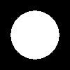
I get:

The edges of the circle are a bit rough since I only used 100 by 100 pixels.

Now it's my turn to do...

1. centered square aperture:
   
2. sinusoid along the x-direction (corrugated roof):
   
3. grating along the x-direction:
   
4. annulus: (from here onwards I used 256 by 256 pixels)
   
5. circular aperture with graded transparency (gaussian transparency):

And aside from these required patterns, I've made some more patterns:

1. Cross
   
2. Double slit
   
3. Half moon
   
4. Smiley
   

The code for all these is:

nx = 256; ny = 256; //defines the number of elements along x and y

x = linspace(-1,1,nx); //defines the range
y = linspace(-1,1,ny);
[X,Y] = ndgrid(x,y); //creates two 2-D arrays of x and y coordinates

Pinhole
r= sqrt(X.^2 + Y.^2); //note element-per-element squaring of X and Y
A = zeros (nx,ny);
A (find(r < 0.7)) = 1;

Centered Square Aperture
A = ones (nx,ny);
A(find(abs(X) > 0.4)) = 0;
A(find(abs(Y) > 0.4)) = 0;

Sinusoid along the x-direction (corrugated roof)
A = ones (nx,ny);
x = 2 * 2 * %pi * linspace(-1, 1, nx);
[X,Y] = ndgrid(x,y);
A = sin(X)
minimum = min(A)
A = (A - minimum)
maximum = max(A)
A = A/maximum

Grating along the x-direction
A = ones (nx,ny);
A(find(abs(X) < 1.1)) = 0;
A(find(abs(X) < 0.9)) = 1;
A(find(abs(X) < 0.7)) = 0;
A(find(abs(X) < 0.5)) = 1;
A(find(abs(X) < 0.3)) = 0;
A(find(abs(X) < 0.1)) = 1;

Annulus
r= sqrt(X.^2 + Y.^2); //note element-per-element squaring of X and Y
A = zeros (nx,ny);
A (find(r < 0.7) ) = 1;
A (find(r < 0.3) ) = 0;

Circular aperture with graded transparency (gaussian transparency)
r= sqrt(X.^2 + Y.^2);
A = exp(-r.^2/0.15)
A(find(r > 0.6)) = 0;

Cross
A = zeros (nx,ny);
A(find(abs(X) < 0.15)) = 1;
A(find(abs(Y) < 0.15)) =1;

Double slit along y
A = zeros (nx,ny);
A(find(abs(Y)<0.25)) = 1;
A(find(abs(Y)<0.15)) = 0;

Half moon
r= sqrt(X.^2 + Y.^2);
A = zeros (nx,ny);
A(find(r < 0.6)) = 1;
A(find(Y > 0)) = 0;

Smiley
r= sqrt(X.^2 + Y.^2);
A = zeros (nx,ny);
A(find(r < 0.5)) =1;
A(find(X < 0)) = 0;
A(find(((X+0.4).^2 + (Y+0.4).^2) < 0.01)) = 1;
A(find(((X+0.4).^2 + (Y-0.4).^2) < 0.01)) = 1;

imshow (A, []);
imwrite(A, 'pinhole.jpg');
imwrite(A, 'centered_square_aperture.jpg');
imwrite(A, 'annulus.jpg');
imwrite(A, 'sinusoid x.jpg');
imwrite(A, 'grating x.jpg');
imwrite(A, 'circ graded transparency.jpg');
imwrite(A, 'cross.jpg');
imwrite(A, "double slit.jpg");
imwrite(A, 'half moon.jpg');
imwrite(A, 'smiley.jpg');

Just comment out segments of the code to produce specific patterns. Grading myself, I would give it a score of perfect 10/10 for being able to produce all the required patterns, for understanding the lesson and presenting the images with proper labels. Plus, a bonus of two points for going beyond the requirements and trying it out with other patterns.

Score: 12/10

Lastly, I want to thank Dr. Soriano, Bayosa Aya Carino and Aivin Solatorio for giving insights and helping me with this activity.


- Dennis Diaz