AP 186 Act10 - Binary Operations

We're back again after a long delay because of SPP hahaha XD

Anyway, in this activity we will be applying the morphological operations as well as the lessons learned in previous activities to determine the best estimate of a cell from an image and then filter out cancer cells later on. :)

So the first part is to determine the best estimate (mean +- stdev) of a normal cell given an image. An image was provided to us wherein the punched papers represent the cells.

Circles

And we were asked to crop this image into 256 x 256 sub images. Here are sample subimages:

sample sub-images

We also cropped out an individual cell to determine it's size:

a normal cell

So we get it's histogram and determine the best value for the threshold in converting it to black and white:

histogram of gray scale values

and we have determined the threshold to be 0.79. Next we convert this image to black and white, and perform opening to close the salt and pepper noise around the cell. Then using what we learned in the Area estimation activity, I determined the cell to have an area of 519 pixels.

However this is not the best estimate for the area, it is just to give us an idea around what value the area is. To determine the best estimate, we loop through every sub-image, convert this to black and white, perform closing to close off the holes inside the cell (due to noise), and then perform opening to remove the salt and pepper noise outside the cells. Then we used bwlabel to identify each blob, and for each blob, we measured the area and tallied them. This was done for all subimages.

The structuring element (strel) for the opening operation is a circle with it's size being a little smaller than the area of the cell. Thus, blobs smaller than this would be erased. Meanwhile the strel used for the closing operation is also a circle but it's size is very small, this is to make the noise or small holes in the cell disappear while minimizing the tendency of closely adjacent blobs to merge due to the closing operation.

Next we plot the histogram of all the tallied areas:

histogram of tallied areas

zooming in to the range around 519... (area of the unit cell:

zoomed-in histogram of tallied areas

but beware! Using too few bins for the histogram would lead to inaccurate estimates for the area. From the above histogram, one might think the range would be 350 - 650 pixels. However, using more bins we see that...

histogram of tallied areas using more bins

and zooming in,

zoomed-in histogram using more bins

We can see that it is now separated into two ranges. Therefore the more accurate range would be around 450 - 650 pixels. We then get the values falling in that range and compute for the mean and standard deviation. The best estimate for the normal cell is 528.96825 +- 25.079209 pixels.

For the next part, we are given another image with some "cells" being bigger than others. These represent cancer cells and we're asked to design and implement a procedure for isolating these cells.

normal cells with cancer cells

So just like in the procedure a while ago, we first determine the best threshold value by getting the histogram of the gray scale image:

histogram of gray scale image

The best threshold is chosen to be 0.845. This is the black and white version of it:

after converting to black and white

Then we cropped out an individual "cancer cell" and determined its size to be 998 pixels. We converted the image to black and white, perform closing and opening:

"cancer cell"

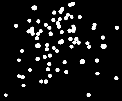after performing closing and opening

and using bwlabel, the areas of all the blobs were tallied and their histogram is:

histogram of tallied areas

We select the range from 950 - 1050 pixels and get their mean and standard deviation. The best estimate of the "cancer cell" is 998.3333 +- 19.033304 pixels.

Next, we loop through every blob and check if its area is within this range, if it is not, the blob is erased. Finally, we obtain the following result:

isolated cancer cells with some blobs of overlapping normal cells

comparing this to the original image, all 5 "cancer cells" were isolated. However, there are also blobs which are just overlaps of two normal cells that are included because their area falls within the range. This is acceptable since this is just the first pass for the filter, additional filters would also examine the shape of these "cells" and distinguish which is which. But nevertheless we have isolated these "cancer cells" using binary operations. :D

For the score, I give myself a 10/10 for producing all the required output and understanding the lesson.

Score : 10/10

And I would like to acknowledge Dr. Soriano, BA Racoma, Theiss Trono, Arvin Mabilangan and Joseph Bunao for the helpful discussions. Thank you :)

- Dennis

References:
1. M. Soriano, "A10 - Binary Operations"

Appendix: Code

Getting threshold value of circles.jpg

A = gray_imread("C:\unitcell.png");
histplot(75, A);

// Set the strel:
nx = 27;
ny = 27;
x = linspace(-1,1,nx);
y = linspace(-1,1,ny);
[X,Y] = ndgrid(x,y);
r = sqrt(X.^2 + Y.^2);
strelopen = zeros (nx,ny);
strelopen(find(r<0.8)) strelclose =" zeros" arealist =" [];" b =" im2bw(A," c =" erode(B," d =" dilate(C," e="="1);" rc =" [r'" s =" size(rc);" unitcellsize =" s(1);" i =" 1:14" a =" gray_imread(" b =" im2bw(A," c =" dilate(B," d =" erode(C," e =" erode(D," f =" dilate(E," i =" 1:n" l="="i);" rc =" [r'" s =" size(rc);" area =" s(1);" arealist =" [Arealist" g =" find(Arealist" h =" Arealist(G);" i =" find(H"> 440);
J = H(I);

// Get the mean and stdev:
ave = mean(J);
sdev = stdev(J);

---------------------------------
For 2nd part:


// Procedure for isolating cancer cells in Circles_with_cancer.jpg
A = gray_imread("C:\Circles_with_cancer.jpg");

//Get histogram of grayscale values:
histplot(75, A);
//Now you have the threshold value. Choose it to be 0.845
threshold = 0.845;


//Get area of cancer unit cell
A = gray_imread("C:\unitcancercell.jpg");
B = im2bw(A, threshold);
C = erode(B, strel, [13, 13]);
D = dilate(C, strel,[13, 13]);
[E, n] = bwlabel(D);
[r, c] = find(E==1);
rc = [r' c'];
s = size(rc);
unitcellsize = s(1);
unitcellsize is determined to be 998 pixels.

B = im2bw(A, threshold);

// Perform closing first
C = dilate(B, strelclose, [14, 14]);
D = erode(C, strelclose, [14,14]);

// Perform opening
E = erode(D, strelopen, [14,14]);
F = dilate(E, strelopen, [14,14]);

[L, n] = bwlabel(F);

for i = 1:n
[r, c] = find(L==i);
rc = [r' c'];
s = size(rc);
Area = s(1);
Arealist = [Arealist Area];
end

histplot(200, Arealist);

// Cancer cell size: 998.3333 +- 19.033304 pixels.

Area_lowerbound = 998.3333 - 19.033304;
Area_upperbound = 998.3333 + 19.033304;

X = zeros(618, 748);

for i = 1:n
[r, c] = find(L==i);
rc = [r' c'];
s = size(rc);
Area = s(1);
if Area > Area_lowerbound then
if Area < Area_upperbound then
X(find(L==i)) = 1;
end
clear rc;
clear s;
clear Area;
end
end

imshow(X,[]);


-----------end-------------