First I pick an image with a single color and I chose this picture which i took:
 picture of a Ferrari to be used for this activity
next we crop a region of interest that is monochromatic...
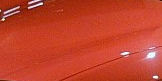 region of interest cropped from the front hood of the car
We first perform the parametric segmentation:
The ROI was loaded into scilab and the RGB colors were transformed into Normalized Chromaticity Coordinates (NCC) then from there the r and g values can be computed. After which we assumed independent Gaussian distributions in r and g and computed for their mean and standard deviation. From here the joint probability function is obtained and this criteria is used to segment the whole image. The result is a grayscale image:
 parametric segmentation of the region of interest (the car)
and one can see that the red body of the car is isolated from the surroundings. The black spots near the front of the car are due to specular reflections in the image so they appear white and were not included. Even the reflection of the car from the glass window is included.
Next we perform another method which is the non-parametric segmentation. This method utilizes the 2D histogram of the r and g values in the ROI. So instead of computing the joint probability per pixel, the method looks up the it's value in the 2D histogram using the pixel's r and g values - backprojection in short. So from the r and g values of the ROI we made the 2D histogram:
 2D histogram of r and g values of ROI
but since its origin is on the top left corner, we rotate this by 90 degrees by using mogrify function:
 rotated 2D histogram of the ROI
 normalized chromaticity space
and comparing this to the rg chromaticity diagram, the peak in the histogram coincide with the reddish part of the normalized chromaticity space which is correct since the ROI is reddish in color. Using this histogram, we performed histogram backprojection which is similar to activity 5 (Enhancement by histogram manipulation) and the result is:
 non-parametric segmentation of the ROI (the car)
Comparing the results of the two methods, I would really have to say that the parametric method worked better at first glance. Nearly the entire body of the car is separated from the background while in non-parametric segmentation, the bumper as well as some other parts of the car are very faint. Although both methods were able to get the reflection of the car from the windows, the result from the parametric method seems to be better and more detailed. Looking at the 1D histograms of r and g value of the ROI...
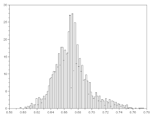 histogram of r values of ROI
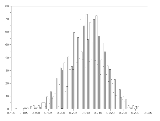 histogram of g values of ROI
To grade myself, I give a 10/10 for comprehending the lesson and producing the required results.
Score: 10/10
Lastly I would like to acknowledge Dr. Soriano for helping me understand more about this activity.
References:
1. M. Soriano, "Color Image Segmentation"
Appendix: (code)
// AP186 Act 12 Color Image Segmentation
ROI = imread("C:\ROI.PNG");
// PARAMETRIC METHOD
// Compute per pixel the r and g values
R = ROI(:,:,1);
G = ROI(:,:,2);
B = ROI(:,:,3);
clear ROI;
divisor = R + G + B;
divisor(find(divisor==0)) = 1000000;
r = R ./ divisor;
g = G ./divisor;
clear R;
clear G;
clear B;
// Get mean and stdev of r ang g:
rmean = mean(r);
gmean = mean(g);
rstdev = stdev(r);
gstdev = stdev(g);
// For the whole image...
A = imread("C:\Ferrari_side_view.JPG");
// Compute per pixel the r and g values
R = A(:,:,1);
G = A(:,:,2);
B = A(:,:,3);
clear A;
divisor = R + G + B;
divisor(find(divisor==0)) = 1000000;
r = R ./ divisor;
g = G ./divisor;
clear R;
clear G;
clear B;
 histogram of r values of ROI
 histogram of g values of ROI
no wonder the results of the parametric method were so good... we assumed r and g to have a gaussian distribution and looking at the histograms above, a gaussian distribution would be a good enough fit.
To grade myself, I give a 10/10 for comprehending the lesson and producing the required results.
Score: 10/10
Lastly I would like to acknowledge Dr. Soriano for helping me understand more about this activity.
References:
1. M. Soriano, "Color Image Segmentation"
Appendix: (code)
// AP186 Act 12 Color Image Segmentation
ROI = imread("C:\ROI.PNG");
// PARAMETRIC METHOD
// Compute per pixel the r and g values
R = ROI(:,:,1);
G = ROI(:,:,2);
B = ROI(:,:,3);
clear ROI;
divisor = R + G + B;
divisor(find(divisor==0)) = 1000000;
r = R ./ divisor;
g = G ./divisor;
clear R;
clear G;
clear B;
// Get mean and stdev of r ang g:
rmean = mean(r);
gmean = mean(g);
rstdev = stdev(r);
gstdev = stdev(g);
// For the whole image...
A = imread("C:\Ferrari_side_view.JPG");
// Compute per pixel the r and g values
R = A(:,:,1);
G = A(:,:,2);
B = A(:,:,3);
clear A;
divisor = R + G + B;
divisor(find(divisor==0)) = 1000000;
r = R ./ divisor;
g = G ./divisor;
clear R;
clear G;
clear B;
// Get their probabilities...
pr = 1/(rstdev * sqrt(2 * %pi)) * exp(-((r - rmean).^2)/(2*(rstdev^2)));
pg = 1/(gstdev * sqrt(2 * %pi)) * exp(-((g - gmean).^2)/(2*(gstdev^2)));
JP = pr .* pg;
//scf();
//imshow(JP, []);
//NON-PARAMETRIC METHOD
// Compute per pixel the r and g values
ROI = imread("C:\ROI.PNG");
R = ROI(:,:,1);
G = ROI(:,:,2);
B = ROI(:,:,3);
clear ROI;
divisor = R + G + B;
divisor(find(divisor==0)) = 1000000;
r = R ./ divisor;
g = G ./divisor;
clear R;
clear G;
clear B;
BINS = 32;
rint = round(r*(BINS-1) + 1); //ranges from 1 to 32
gint = round(g*(BINS-1) + 1);
colors = gint(:) + (rint(:)-1)*BINS;
hist = zeros(BINS, BINS);
for row = 1:BINS
for col = 1:(BINS-row+1)
hist(row, col) = length(find(colors==( ((col + (row-1)*BINS)))));
end;
end;
//scf();
//histmax = max(hist);
//X = hist/histmax;
//Y = mogrify(X, ['-rotate', '-90']);
//imshow(Y, []);
// For the whole image...
A = imread("C:\Ferrari_side_view.JPG");
// Compute per pixel the r and g values
R = A(:,:,1);
G = A(:,:,2);
B = A(:,:,3);
clear A;
divisor = R + G + B;
divisor(find(divisor==0)) = 1000000;
r = R ./ divisor;
g = G ./divisor;
clear R;
clear G;
clear B;
//Backproject
s = size(r);
rows = s(1);
columns = s(2);
S = zeros(rows, columns);
for i=1:rows
for j=1:columns
rvalue = r(i, j);
gvalue = g(i, j);
// round off since hist has only 32 bins
rint = round(rvalue*(BINS-1) + 1);
gint = round(gvalue*(BINS-1) + 1);
value = hist(rint, gint);
// replace pixel with the value
S(i, j) = value;
end;
end;
imshow(S, []);
--------------------------end-----------------------
No comments:
Post a Comment